Estimating number of transcripts from RNA-Seq measurements (and why I believe in paywall)

I was recently reading the latest ENCODE paper published in PNAS when a sentence in the caption of Figure 2 caught my attention:

“Depending on the total amount of RNA in a cell, one transcript copy per cell corresponds to between 0.5 and 5 FPKM in PolyA+ whole-cell samples according to current estimates (with the upper end of that range corresponding to small cells with little RNA and vice versa).”

Although very few people actually care about ENCODE, many people do care about the interpretation of RNA-Seq FPKM measurements and to them this is likely to be a sentence of interest. In fact, there have been a number of attempts to provide intuitive meaning for RPKM (and FPKM) in terms of copy numbers of transcripts per cell. Even though the ENCODE PNAS paper provides no citation for the statement (or methods section explaining the derivation), I believe its source is the RNA-Seq paper by Mortazavi et al. In that paper, the authors write that

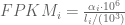
“…absolute transcript levels per cell can also be calculated. For example, on the basis of literature values for the mRNA content of a liver cell [Galau et al. 1977] and the RNA standards, we estimated that 3 RPKM corresponds to about one transcript per liver cell. For C2C12 tissue culture cells, for which we know the starting cell number and RNA preparation yields needed to make the calculation, a transcript of 1 RPKM corresponds to approximately one transcript per cell. “

This statement has been picked up on in a number of publications (e.g., Hebenstreit et al., 2011, van Bakel et al., 2011). However the inference of transcript copies per cell directly from RPKM or FPKM estimates is not possible and conversion factors such as 1 RPKM = 1 transcript per cell are incoherent. At the same time, the estimates of Mortazavi et al. and the range provided in the ENCODE PNAS paper are informative. The “incoherence” stems from a subtle issue in the normalization of RPKM/FPKM that I have discussed in a talk I gave at CSHL, and is the reason why TPM is a better unit for RNA abundance. Still, the estimates turn out to be “informative”, in the sense that the effect of (lack of) normalization appears to be smaller than variability in the amount of RNA per cell. I explain these issues below:

Why is the sentence incoherent?

RNA-Seq can be used to estimate transcript abundances in an RNA sample. Formally, a sample consists of n distinct types of transcripts, and each occurs with different multiplicity (copy number), so that transcript i appears times in the sample. By “abundance” we mean the relative amounts where . Note that   and . Suppose that for some j. The corresponding is therefore where . The question is what does this value correspond to in RPKM (or FPKM).

RPKM stands for “reads per kilobase  of transcript per million reads mapped” and FPKM is the same except with “fragment” replacing read (initially reads were not paired-end, but with the advent of paired-end sequencing it makes more sense to speak of fragments, and hence FPKM). As a unit of measurement for an estimate, what FPKM really refers to is the expected number of fragments per kilboase of transcript per million reads. Formally, if we let be the length of transcript i and define then abundance in FPKM for transcript i is abundance measured as . In terms of , we obtain that

.

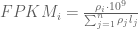
The term in the denominator can be considered a kind of normalization factor, that while identical for each transcript, depends on the abundances of each transcript (unless all lengths are equal). It is in essence an average of lengths of transcripts weighted by abundance. Moreover, the length of each transcript should be taken to be taken to be its “effective” length, i.e. the length with respect to fragment lengths, or equivalently, the number of positions where fragments can start.

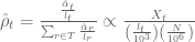
The implication for finding a relationship between FPKM and relative abundance constituting one transcript copy per cell is that one cannot. Mathematically, the latter is equivalent to setting in the formula above and then trying to determine . Unfortunately, all the remaining are still in the formula, and must be known in order to calculate the corresponding FPKM value.

The argument above makes clear that it does not make sense to estimate transcript copy counts per cell in terms of RPKM or FPKM. Measurements in RPKM or FPKM units depend on the abundances of transcripts in the specific sample being considered, and therefore the connection to copy counts is incoherent. The obvious and correct solution is to work directly with the . This is the rationale of TPM (transcripts per million) used by Bo Li and Colin Dewey in the RSEM paper (the argument for TPM is also made in Wagner et al. 2012).

Why is the sentence informative?

Even though incoherent, it turns out there is some truth to the ranges and estimates of copy count per cell in terms of RPKM and FPKM that have been circulated. To understand why requires noting that there are in fact two factors that come into play in estimating the FPKM corresponding to abundance of one transcript copy per cell. First, is M as defined above to be the total number of transcripts in a cell. This depends on the amount of RNA in a cell. Second are the relative abundances of all transcripts and their contribution to the denominator in the formula.

The best paper to date on the connection between transcript copy numbers and RNA-Seq measurements is the careful work of Marinov et al. in “From single-cell to cell-pool transcriptomes: stochasticity in gene expression and RNA splicing” published in Genome Research earlier this year. First of all, the paper describes careful estimates of RNA quantities in different cells, and concludes that (at least for the cells studied in the paper) amounts vary by approximately one order of magnitude. Incidentally, the estimates in Marinov et al. confirm and are consistent with rough estimates of Galau et al. from 1977, of 300,000 transcripts per cell. Marinov et al. also use spike-in measurements are used to conclude that in “GM12878 single cells, one transcript copy corresponds to ∼10 FPKM on average.”. The main value of the paper lies in its confirmation that RNA quantities can vary by an order of magnitude, and I am guessing this factor of 10 is the basis for the range provided in the ENCODE PNAS paper (0.5 to 5 FPKM).

In order to determine the relative importance of the denominator in I looked at a few RNA-Seq datasets we are currently examining. In the GEUVADIS data, the weighted average can vary by as much as 20% between samples. In a rat RNA-Seq dataset we are analyzing, the difference is a factor of two (and interestingly very dependent on the exact annotation used for quantification). The point here is that even the denominator in  does vary, but less, it seems, than the variability in RNA quantity. In other words, the estimate of 0.5 to 5 FPKM corresponding to one transcript per cell is incoherent albeit probably not too far off.

One consequence of all of the above discussion is that while differential analysis of experiments can be performed based on FPKM units (as done for example in Cufflinks, where the normalization factors are appropriately accounted for), it does not make sense to compare raw FPKM values across experiments. This is precisely what is done in Figure 2 of the ENCODE PNAS paper. What the analysis above shows, is that actual abundances may be off by amounts much larger than the differences shown in the figure. In other words, while the caption turns out to contain an interesting comment the overall figure doesn’t really make sense. Specifically, I’m not sure the relative RPKM values shown in the figure deliver the correct relative amounts, an issue that ENCODE can and should check. Which brings me to the last part of this post…

What is ENCODE doing?

Having realized the possible issue with RPKM comparisons in Figure 2, I took a look at Figure 3 to try to understand whether there were potential implications for it as well. That exercise took me to a whole other level of ENCODEness. To begin with, I was trying to make sense of the x-axis, which is labeled “biochemical signal strength (log10)” when I realized that the different curves on the plot all come from different, completely unrelated x-axes. If this sounds confusing, it is. The green curves are showing graphs of functions whose domain is in log 10 RPKM units. However the histone modification curves are in log (-10 log p), where p is a p-value that has been computed. I’ve never seen anyone plot log(log(p-values)); what does it mean?! Nor do I understand how such graphs can be placed on a common x-axis (?!). What is “biochemical signal strength” (?) Why in the bottom panel is the grey H3K9me3 showing %nucleotides conserved decreasing as “biochemical strength” is increasing (?!) Why is the green RNA curves showing conservation below genome average for low expressed transcripts (?!) and why in the top panel is the red H3K4me3 an “M” shape (?!) What does any of this mean (?!) What I’m supposed to understand from it, or frankly, what is going on at all ??? I know many of the authors of this ENCODE PNAS paper and I simply cannot believe they saw and approved this figure. It is truly beyond belief… see below:

All of these figures are of course to support the main point of the paper. Which is that even though 80% of the genome is functional it is also true that this is not what was meant to be said , and that what is true is that “survey of biochemical activity led to a significant increase in genome coverage and thus accentuated the discrepancy between biochemical and evolutionary estimates… where function is ascertained independently of cellular state but is dependent on environment and evolutionary niche therefore resulting in estimates that  differ widely in their false-positive and false-negative rates and the resolution with which elements can be defined… [unlike] genetic approaches that rely on sequence alterations to establish the biological relevance of a DNA segment and are often considered a gold standard for defining function.”

Alright then.

The ENCODE PNAS paper was first published behind a paywall. However after some public criticism, the authors relented and paid for it to be open access. This was a mistake. Had it remained behind a paywall not only would the consortium have saved money, I and others might have been spared the experience of reading the paper. I hope the consortium will afford me the courtesy of paywall next time.

Don’t believe the Affymetrix anti-hype

Don’t believe the anti-hype. They are saying that RNA-Seq promises the discovery of new expression events, but it doesn’t deliver:

Is this true? There have been a few papers comparing microarrays to RNA-Seq technology (including one of my own) that I’ll discuss below, but first a break-down of the Affymetrix “evidence”. The first is this figure (the poor quality of the images is exactly what Affymetrix provides, and not due to a reduction in quality on this site; they are slightly enlarged when clicked on):

The content of this figure is an illustration of the gene LMNB1 (Lamin protein of type B), used to argue that microarrays can provide transcript level resolution whereas RNA-Seq can’t!! Really? Affymetrix is saying that RNA-Seq users would likely use the RefSeq annotation which only has three isoforms. But this is a ridiculous claim. It is well known that RefSeq is a conservative annotation and certainly RNA-Seq users have the same access to the multiple databases Affymetrix used to build their annotation (presumably, e.g. Ensembl). It therefore seems that what Affymetrix is saying with this figure is that RNA-Seq users are dumb.

The next figure is showing the variability in abundance estimates as a function of expression level for RNA-SEq and the HTA 2.0, with the intended message being that microarrays are less noisy:

But there is a subtle trick going on here. And its in the units. The x-axis is showing RPM, which is an abbreviation for Reads Per Million. This is not a commonly used unit, and there is a reason. First, its helpful to review what is used. In his landmark paper on RNA-Seq, Ali Mortazavi introduced the units RPKM (note the extra K) that stands for reads per kilobase of transcript per million mapped. Why the extra kilobase term? In my review on RNA-Seq quantification I explain that RPKM is proportional to a maximum likelihood estimate of transcript abundance (obtained from a simple RNA-Seq model). The complete derivation is on page 6 ending in Equation 13; I include a summary here:

The maximum likelihood (ML) abundances  are  given by

In these equations is the length of transcript t (if reads are long it is necessary to modify the length due to edge effects, hence the tilde in the paper), the are the maximum likelihood estimates for the probabilities of selecting reads from transcripts (unnormalized by their length) and finally is the number of reads mapping to transcript t while N is the total number of mapped reads. The point is that RPKM (the rightmost formula for abundance) is really a unit for describing the maximum likelihood relative abundances () scaled by some factors.

RPKM as a unit has two problems. The first is that in current RNA-Seq experiments reads are paired so that the actual units being counted (in ) are fragments. For this reason we modified RPKM to FPKM in the Cufflinks paper (the “F” replaced “R” for fragment instead of read). A more serious problem, noted by Bo Li and Colin Dewey in their paper on RSEM, is that while FPKM is proportional to ML estimates of abundance, the proportionality constants may vary between experiments. For this reason they proposed TPM (transcripts per million) which is also proportional to the ML abundance estimates but with a proportionality constant (a million) that is the same between experiments. All of these units are used simply to avoid writing down the which are in many cases tiny numbers since they must all sum to 1.

Returning to the Affymetrix figure, we see the strange RPM units. In essence, this is the rightmost term in the equation above, with the length terms removed from the denominators. Therefore RPM is proportional to the . If a transcript is short, even if it is equally abundant to a longer transcript ,it will produce less RNA-Seq reads and therefore its will be (possibly considerably) smaller. The effect of displaying RPM for RNA-Seq vs. expression level for the HTA 2.0 arrays is therefore to mix apples and oranges. Since what is being displayed is a coefficient of variation, there is a bias caused by the relationship between length and expression (e.g. many highly expressed housekeeping genes are short).

To be fair to Affymetrix the conversion between the and the can be confusing (its explained in Lemma 14 in the Supplement of the Cufflinks paper). So maybe the discordant x-axes were unintentional…but then there is the third figure:

Here its a bit hard to tell what is going on because not all the information needed to decipher the figure is provided. For example, its not clear how the “expression of exons” was computed or measured for the RNA-Seq experiment. I suspect that as with the previous figure, read numbers were not normalized by length of exons, and moreover spliced reads (and other possibly informative reads from transcripts) were ignored. In other words, I don’t really believe the result.

Having said this, it is true that expression arrays can have an advantage in measuring exon expression, because an array measurement is absolute (as opposed to the relative quantification that is all that is possible with RNA-Seq). Array signal is based on hybridization, and it is probably a reasonable assumption that some minimum amount of RNA triggers a signal, and that this amount is independent of the remainder of the RNA in an experiment. So arrays can (and in many cases probably do) have advantages over RNA-Seq.

There are a few papers that have looked into this, for example the paper “A comprehensive comparison of RNA-Seq-based transcriptome analysis from reads to differential gene expression and cross-comparison with microarrays: a case study in Saccharomyces cerevisiae ” by Nookaew et al., Nucleic Acids Research 40 (2012) who find high reproducibility in RNA-Seq and consistency between arrays and RNA-Seq.  Xu et al., in “Human transcriptome array for high-throughput clinical studies“, PNAS 108 (2011), 3707–3712 are more critical, agreeing with Affymetrix that arrays are more sensitive at the exon level. For disease studies, they recommend using RNA-Seq to identify transcripts relevant to the disease, and then screening for those transcripts on patients using arrays.

For the Cuffdiff2 paper describing our new statistical procedures for differential analysis of transcripts and genes, the Rinn lab performed deep RNA-Seq and array expression measurement on the same samples from a HOXA1 knowdown (the experiments included multiple replicates of both the RNA-Seq and the arrays). To my knowledge, it is the deepest and most comprehensive data currently available for comparing arrays and RNA-Seq. Admittedly, the arrays used were not Affymetrix but Agilent SurePrint G3, and the RNA-Seq coverage was deep, however we had two main findings very different from the Affymetrix claims. First, we found overall strong correlation between array expression values and RNA-Seq abundance estimates. The correlation remained strong for large regimes of expression even with very few reads (tested by sequencing fewer reads from a MiSeq). Second, we found that arrays were missing differentially expressed transcripts, especially at low abundance levels. In other words, we found RNA-Seq to have higher resolution. The following figure from our paper made the case (note the overall Spearman Correlation was 0.86):

There are definitely continued applications for arrays. Both in high-throughput screening applications (as suggested in the Xu et al. paper), and also in the development of novel assays. For example Mercer et al. “Targeted rNA sequencing reveals the deep complexity of the human transcriptome“, Nature Biotechnology 30 (2012) 99–104  show how to couple capture (with arrays) with RNA-Seq to provide ultra deep sequencing in subsets of the transcriptome. So its not yet the time to write off arrays. But RNA-Seq has many applications of its own. For example the ability to better detect allele-specific expression, the opportunity to identify RNA-DNA differences (and thereby study RNA editing), and the ability to study expression in non-model organisms where genomes sequences are incomplete and annotations poor. For all these reasons I’m betting on RNA-Seq.