Fast and accurate gene differential expression by testing transcript compatibility counts

This post is a review of a recent preprint on an approach to testing for RNA-seq gene differential expression directly from transcript compatibility counts:

Marek Cmero, Nadia M Davidson and Alicia Oshlack, Fast and accurate differential transcript usage by testing equivalence class counts, bioRxiv 2018.

To understand the preprint two definitions are important. The first is of gene differential expression, which I wrote about in a previous blog post and is best understood, I think, with the following figure (reproduced from Supplementary Figure 1 of Ntranos, Yi, et al., 2018):

In this figure, two isoforms of a hypothetical gene are called primary and secondary, and two conditions in a hypothetical experiment are called “A” and “B”. The black dots labeled conditions A and B have x-coordinates  and  corresponding to the abundances of the primary isoform in the respective conditions, and y-coordinates  and  corresponding to the abundance of the secondary isoforms. In data from the hypothetical experiment, the black dots represent the mean level of expression of the constituent isoforms as derived from replicates. Differential transcript expression (DTE) refers to change in one of the isoforms. Differential gene expression (DGE) refers to change in overall gene expression (i.e. expression as the sum of the expression of the two isoforms). Differential transcript usage (DTU) refers to change in relative expression between the two isoform and gene differential expression (GDE) refers to change in expression along the red line. Note that DGE, DTU and DGE are special cases of GDE.

The Cmero et al. preprint describes a method for testing for GDE, and the method is based on comparison of equivalence classes of reads between conditions. There is a natural equivalence relation on the set of reads in an RNA-seq experiment, where two reads and are related by when and align (ambiguously) to exactly the same set of transcripts (see, e.g. Nicolae et al. 2011). The equivalence relation partitions the reads into equivalence classes, and, in a slight abuse of notation, the term “equivalence class” in RNA-seq is used to denote the set of transcripts corresponding to an equivalence class of reads. Starting with the pseudoalignment program kallisto published in Bray et al. 2016, it became possible to rapidly obtain the (transcript) equivalence classes for reads from an RNA-seq experiment.

In previous work (Ntranos et al. 2016) we introduced the term transcript compatibility counts to denote the cardinality of the (read) equivalence classes. We thought about this name carefully; due to the abuse of notation inherent in the term “equivalence class” in RNA-seq, we felt that using “equivalence class counts” would be confusing as it would be unclear whether it refers to the cardinalities of the (read) equivalence classes or the (transcript) “equivalence classes”.

With these definitions at hand, the Cmero et al.’s preprint can be understood to describe a method for identifying GDE between conditions by directly comparing transcript compatibility counts. The Cmero et al. method is to perform Šidák aggregation of p-values for equivalence classes, where the p-values are computed by comparing transcript compatibility counts for each equivalence class with the program DEXSeq (Anders et al. 2012). A different method that also identifies GDE by directly comparing transcript compatibility counts was previously published by my student Lynn Yi in Yi et al. 2018. I was curious to see how the Yi et al. method, which is based on Lancaster aggregation of p-values computed from transcript compatibility counts compares to the Cmero et al. method. Fortunately it was really easy to find out because Cmero et al. released code with their paper that can be used to make all of their figures.

I would like to note how much fun it is to reproduce someone else’s work. It is extremely empowering to know that all the methods of a paper are pliable at the press of a button. Below is the first results figure, Figure 2, from Cmero et al.’s paper:

Below is the same figure reproduced independently using their code (and downloading the relevant data):

It’s beautiful to see not only apples-to-apples, but the exact same apple! Reproducibility is obviously important to facilitate transparency in papers and to ensure correctness, but its real value lies in the fact that it allows for modifying and experimenting with methods in a paper. Below is the second results figure, Figure 3, from Cmero et al.’s paper:

The figure below is the reproduction, but with an added analysis in Figure 3a, namely the method of Yi et al. 2018 included (shown in orange as “Lancaster_equivalence_class”).

The additional code required for the extra analysis is just a few lines and can be downloaded from the Bits of DNA Github repository:

---

library(aggregation)
library(dplyr)
dm_dexseq_results <- as.data.frame(DEXSeqResults(dm_ec_results$dexseq_object))
dm_lancaster_results <- dm_dexseq_results %>% group_by(groupID) %>% summarize(pval = lancaster(pvalue, log(exonBaseMean)))
dm_lancaster_results$gene_FDR <- p.adjust(dm_lancaster_results$pval, ‘BH’)
dm_lancaster_results <- data.frame(gene = dm_lancaster_results$groupID,
FDR = dm_lancaster_results$gene_FDR)

hs_dexseq_results <- as.data.frame(DEXSeqResults(hs_ec_results$dexseq_object))
hs_lancaster_results <- hs_dexseq_results %>% group_by(groupID) %>% summarize(pval = lancaster(pvalue, log(exonBaseMean)))
hs_lancaster_results$gene_FDR <- p.adjust(hs_lancaster_results$pval, ‘BH’)
hs_lancaster_results <- data.frame(gene = hs_lancaster_results$groupID,
FDR = hs_lancaster_results$gene_FDR)

---

A zoom-in of Figure 3a below shows that the improvement of Yi et al.’s method in the hsapiens dataset over the method of Cmero et al. is as large as the improvement of aggregation (of any sort) over GDE based on transcript quantifications. Importantly, this is a true apples-to-apples comparison because Yi et al.’s method is being tested on exactly the data and with exactly the metrics that Cmero et al. chose:

The improvement is not surprising; an extensive comparison of Lancaster aggregation with Šidák aggregation is detailed in Yi et al. and there we noted that while Šidák aggregation performs well when transcripts are perturbed independently, it performs very poorly in the more common case of correlated effect. Furthermore, we also examined in detail DEXSeq’s aggregation (perGeneQvalue) which appears to be an attempt to perform Šidák aggregation but is not quite right, in a sense we explain in detail in Section 2 of the Yi et al. supplement. While DEXSeq’s implementation of Šidák aggregation does control the FDR, it will tend to report genes with many isoforms and consumes the “FDR budget” faster than Šidák aggregation. This is one reason why, for the purpose of comparing Lancaster and Šidák aggregation in Yi et al. 2018, we did not rely on DEXSeq’s implementation of Šidák aggregation. Needless to say, separately from this issue, as mentioned above we found that Lancaster aggregation substantially outperforms Šidák aggregation.

The figures below complete the reproduction of the results of Cmero et al. The reproduced figures are are very similar to Cmero et al.’s figures but not identical. The difference is likely due to the fact that the Cmero paper states that a full comparison of the “Bottomly data” (on which these results are based) is a comparison of 10 vs. 10 samples. The reproduced results are based on downloading the data which consists of 10 vs. 11 samples for a total of 21 samples (this is confirmed in the Bottomly et al. paper which states that they “generated single end RNA-Seq reads from 10 B6 and 11 D2 mice.”) I also noticed one other small difference in the Drosophila analysis shown in Figure 3a where one of the methods is different for reasons I don’t understand. As for the supplement, the Cmero et al. figures are shown on the left hand side below, and to their right are the reproduced figures:

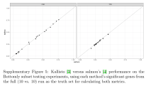
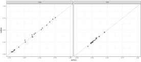
The final supplementary figure is a comparison of kallisto to Salmon: the Cmero et al. paper shows that Salmon results are consistent with kallisto results shown in Figure 3a,  and reproduces the claim I made in a previous blog post, namely that Salmon results are near identical to kallisto:

The final paragraph in the discussion of Cmero et al. states that “[transcript compatibility counts] have the potential to be useful in a range of other expression analysis. In particular [transcript compatibility counts] could be used as the initial unit of measurement for many other types of analysis such as dimension reduction visualizations, clustering and differential expression.” In fact, transcript compatibility counts have already been used for all these applications and have been shown to have numerous advantages. See the papers:

• Ntranos et al. 2016: Demonstrates advantages of clustering single-cell RNA-seq data directly with transcript compatibility counts rather than gene counts.
• Yi et al. 2018: Shows how to perform gene differential expression directly from transcript compatibility counts for bulk RNA-seq data.
• Ntranos, Yi, et al., 2018: Shows that logistic regression with transcript compatibility counts is a powerful approach to gene differential expression from single-cell RNA-seq data.
• Melsted et al. 2018: A new file format for single-cell RNA-seq based on equivalence classes that facilitates fast and accurate processing of single-cell RNA-seq data. This allows for very fast calculation of transcript compatibility counts for the applications above.

Many of these papers were summarized in a talk I gave at Cold Spring Harbor in 2017 on “Post-Procrustean Bioinformatics”, where I emphasized that instead of fitting methods to the predominant data types (in the case of RNA-seq, gene counts), one should work with data types that can support powerful analysis methods (in the case of RNA-seq, transcript compatibility counts).