
[Update July 15, 2016: A preprint describing sleuth is available on BioRxiv]
Today my student Harold Pimentel released the beta version of his new RNA-Seq analysis method and software program called sleuth. A sleuth for RNA-Seq begins with the quantification of samples with kallisto, and together a sleuth of kallistos can be used to analyze RNA-Seq data rigorously and rapidly.

Why do we need another RNA-Seq program?
A major challenge in transcriptome analysis is to determine the transcripts that have changed in their abundance across conditions. This challenge is not entirely trivial because the stochasticity in transcription both within and between cells (biological variation), and the randomness in the experiment (RNA-Seq) that is used to determine transcript abundances (technical variation), make it difficult to determine what constitutes “significant” change.
Technical variation can be assessed by performing technical replicates of experiments. In the case of RNA-Seq, this can be done by repeatedly sequencing from one cDNA library. Such replicates are fundamentally distinct from biological replicates designed to assess biological variation. Biological replicates are performed by sequencing different cDNA libraries that have been constructed from repeated biological experiments performed under the same (or in practice near-same) conditions. Because biological replicates require sequencing different cDNA libraries, a key point is that biological replicates include technical variation.
In the early days of RNA-Seq a few papers (e.g. Marioni et al. 2008, Bullard et al. 2010) described analyses of technical replicates and concluded that they were not really needed in practice, because technical variation could be predicted statistically from the properties of the Poisson distribution. The point is that in an idealized RNA-Seq experiment counts of reads are multinomial (according to abundances of the transcripts they originate from), and therefore approximately Poisson distributed. Their variance is therefore approximately equal to the mean, so that it is possible to predict the variance in counts across technical replicates based on the abundance of the transcripts they originate from. There is, however, one important subtlety here: “counts of reads” as used above refers to the number of reads originating from a transcript, but in many cases, especially in higher eukaryotes, reads are frequently ambiguous as to their transcript of origin because of the presence of multi-isoform genes and genes families. In other words, transcript counts cannot be precisely measured. However, the statement about the Poisson distribution of counts in technical replicates remain true when considering counts of reads by genomic features because then reads are no longer ambiguous.
This is why, in so-called “count-based methods” for RNA-Seq analysis, there is an analysis only at the gene level. Programs such as DESeq/DESeq2, edgeR and a literally dozens of other count-based methods first require counting reads across genome features using tools such as HTSeq or featureCounts. By utilizing read counts to genomic features, technical replicates are unnecessary in lieu of the statistical assumption that they would reveal Poisson distributed data, and instead the methods focus on modeling biological variation. The issue of how to model biological variation is non-trivial because typically very few biological replicates are performed in experiments. Thus, there is a need for pooling information across genes to obtain reliable variance estimates via a statistical process called shrinkage. How and what to shrink is a matter of extensive debate among statisticians engaged in the development of count-based RNA-Seq methods, but one theme that has emerged is that shrinkage approaches can be compatible with general and generalized linear models, thus allowing for the analysis of complex experimental designs.
Despite these accomplishments, count-based methods for RNA-Seq have two major (related) drawbacks: first, the use of counts to gene features prevents inference about the transcription of isoforms, and therefore with most count-based methods it is impossible to identify splicing switches and other isoform changes between conditions. Some methods have tried to address this issue by restricting genomic features to specific exons or splice junctions (e.g. DEXSeq) but this requires throwing out a lot of data, thereby reducing power for identifying statistically significant differences between conditions. Second, because of the fact that in general 
While reads might be ambiguous as to exactly which transcripts they originated from, it is possible to statistically infer an estimate of the number of reads from each transcript in an experiment. This kind of quantification has its origin in papers of Jiang and Wong, 2009 and Trapnell et al. 2010. However the process of estimating transcript-level counts introduces technical variation. That is to say, if multiple technical replicates were performed on a cDNA library and then transcript-level counts were to be inferred, those inferred counts would no longer be Poisson distributed. Thus, there appears to be a need for performing technical replicates after all. Furthermore, it becomes unclear how to work within the shrinkage frameworks of count-based methods.
There have been a handful of attempts to develop methods that combine the uncertainty of count estimates at the transcript level with biological variation in the assessment of statistically significant changes in transcript abundances between conditions. For example, the Cuffdiff2 method generalizes DESeq while the bitSeq method relies on a Bayesian framework to simultaneously quantify abundances at the transcript level while modeling biological variability. Despite showing improved performance over count-based methods, they also have significant shortcomings. For example the methods are not as flexible as those of general(ized) linear models, and bitSeq is slow partly because it requires MCMC sampling.
Thus, despite intensive research on both statistical and computational methods for RNA-Seq over the past years, there has been no solution for analysis of experiments that allows biologists to take full advantage of the power and resolution of RNA-Seq.
The sleuth model
The main contribution of sleuth is an intuitive yet powerful model for RNA-Seq that bridges the gap between count-based methods and quantification algorithms in a way that fully exploits the advantages of both.
To understand sleuth, it is helpful to start with the general linear model:
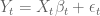
Here the subscript t refers to a specific transcript, 


In the sleuth model the 

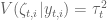
where the 
The sleuth model incorporates the assumptions that the response error is additive, i.e. if the variance of transcript t in sample i is 


In a test of sleuth on data simulated according to the DESeq2 model we found that sleuth significantly outperforms other methods:

In this simulation transcript counts were simulated according to a negative binomial distribution, following closely the protocol of the DESeq2 paper simulations. Reference parameters for the simulation were first estimated by running DESeq2 on a the female Finnish population from the GEUVADIS dataset (59 individuals). In the simulation above size factors were set to be equal in accordance with typical experiments being performed, but we also tested sleuth with size factors drawn at random with geometric mean of 1 in accordance with the DESeq2 protocol (yielding factors of 1, 0.33, 3, 3, 0.33 and 1) and sleuth still outperformed other methods.
There are many details in the implementation of sleuth that are crucial to its performance, e.g. the approach to shrinkage to estimate the biological variance 
Exploratory data analysis with sleuth
One of the design goals of sleuth was to create a simple and efficient workflow in line with the principles of kallisto. Working with the Shiny web application framework we have designed an html interface that allows users to interact with sleuth plots allowing for real time exploratory data analysis.
The sleuth Shiny interface is much more than just a GUI for making plots of kallisto processed data. First, it allows for the exploration of the sleuth fitted models; users can explore the technical variation of each transcript, see where statistically significant differential transcripts appear in relationship to others in terms of abundance and variance and much more. Particularly useful are interactive features in the plots. For example, when examining an MA plot, users can highlight a region of points (dynamically created box in upper panel) and see their variance breakdown of the transcripts the points correspond to, and the list of the transcripts in a table below:

The web interface contains diagnostics, summaries of the data, “maps” showing low-dimensional representations of the data and tools for analysis of differential transcripts. The interactivity via Shiny can be especially useful for diagnostics; for example, in the diagnostics users can examine scatterplots of any two samples, and then select outliers to examine their variance, including the breakdown of technical variance. This allows for a determination of whether outliers represent high variance transcripts, or specific samples gone awry. Users can of course make figures showing transcript abundances in all samples, including boxplots displaying the extent of technical variation. Interested in the differential transcribed isoform ENST00000349155 of the TBX3 gene shown in Figure 5d of the Cuffdiff2 paper? It’s trivial to examine using the transcript viewer:

One can immediately see visually that differences between conditions completely dominate both the technical and biological variation within conditions. The sleuth q-value for this transcript is 3*10^(-68).
Among the maps, users can examine PCA projections onto any pair of components, allowing for rapid exploration of the structure of the data. Thus, with kallisto and sleuth raw RNA-Seq reads can be converted into a complete analysis in a matter of minutes. Experts will be able to generate plots and analyses in R using the sleuth library as they would with any R package. We plan numerous improvements and developments to the sleuth interface in the near future that will further facilitate data exploration; in the meantime we welcome feedback from users.
How to try out sleuth
Since sleuth requires the bootstraps and quantifications output by kallisto we recommend starting by running kallisto on your samples. The kallisto program is very fast, processing 30 million reads on a laptop in a matter of minutes. You will have to run kallisto with bootstraps- we have been using 100 bootstraps per sample but it should be possible to work with many fewer. We have yet to fully investigate the minimum number of bootstraps required for sleuth to be accurate.
To learn how to use kallisto start here. If you have already run kallisto you can proceed to the tutorial for sleuth. If you’re really eager to see sleuth without first learning kallisto, you can skip ahead and try it out using pre-computed kallisto runs of the Cuffdiff2 data- the tutorial explains where to obtain the data for trying out sleuth.
For questions, suggestions or help see the program websites and also the kallisto-sleuth user group. We hope you enjoy the tools!

38 comments
Comments feed for this article
August 17, 2015 at 2:38 pm
Anshul Kundaje
This is awesome. Is there support for adding in or accounting for covariates representing observed or hidden confounding factors? If not, do you plan to add this extension in the future. In my experience, this is a major drawback of many of the multi-sample differential analysis tools in that they do not integrate seamlessly with some of the confounding factor estimation and correction tools. It would be a fantastic addition to this tool. I’m looking forward to testing this out.
August 17, 2015 at 3:00 pm
haroldpimentel
Hi Anshul,
We currently support arbitrary designs for fixed-effects. This means you can condition on batch effects and still measure the ‘fold-change’ between conditions.
Best,
Harold
August 17, 2015 at 6:03 pm
Anshul Kundaje
Great. Thanks.
August 17, 2015 at 6:44 pm
Katja Hebestreit
This sounds great!! I have been using Kallisto and I am really impressed by its speed and its results. I am looking forward to give sleuth a try.
I have 2 questions:
1) How does sleuth behave if the data set has lots of dropout events? In the analysis of single-cell RNA-seq data one is confronted with lots of genes that have a moderate or even high expression level in some cells, but were not detected in other cells. I experienced that these dropouts can lead to a dramatic increase of the false discovery rate for some of the “classic” tools, such as edgeR. It would be super interesting to know how sleuth can deal with those challenges that are specific to single-cell data.
2) Were you guys thinking about submitting this package to Bioconductor? I know it is work, but it is just super convenient for users. It might also push its publicity as you can announce the package through the Bioc mailing list addressing probably hundreds of potential users.
August 18, 2015 at 7:33 am
Valentine Svensson
Katja, don’t you have so many samples in each condition for single-cell data that you can just use e.g. non-parametric tests?
August 18, 2015 at 10:38 am
Katja Hebestreit
That is actually a good idea. I will definitely consider this.
August 18, 2015 at 9:34 am
haroldpimentel
Hi Katja,
Thanks for your interest.
1.) I wouldn’t expect it to do much better than existing methods for dropouts as we do not explicitly model them. However, in our simulations and some datasets we’ve tested we seem to have higher sensitivity due to the modeling of the technical variance. That being said, we’ve actually been thinking a fair bit about scRNA-Seq in this context and will be extending the model as soon as we’ve stabilized sleuth for bulk RNA-Seq.
2.) We’ve been thinking about where to submit it. I’ll take a look at BioC requirements over this week. I definitely agree the BioC community is a great resource.
August 18, 2015 at 10:23 am
MB
How would you model technical variance for single cell? There aren’t technical reps (each cell can only be sequenced once) and for low input RNA seq (which is probably the closest) Poisson models often break because of the PCR cycles and dropouts.
Do you have a sense at the rep cutoff for which there is improved estimates of variance with your method? i.e with 2 reps information sharing usually helps. For 7 or 8 reps just measuring the variance is usually more accurate (in other methods)
Thanks
August 18, 2015 at 10:36 am
Katja Hebestreit
Thank you, Harold! Good luck with it!!
September 4, 2015 at 9:51 am
Alexander Predeus
There are actual methods for single cell RNA-seq differential expression analysis, such as SCDE. Of course it would have been very nice to not have to align SC data, since there’s usually so much of it. You have to consider the UMI barcoding too since SC is so much more sensitive to PCR replication errors.
August 18, 2015 at 8:05 am
James Eales
Very glad you support arbitrary designs, so much flexibility now. I was wondering how you were going to use the bootstraps effectively. I’m off to show my data to a collection of members of the family Ursidae.
August 28, 2015 at 7:09 am
Eduardo Eyras
Hi. Can Sleuth distinguish differential transcripts that do not change total gene output vs those that do? The former would be possibly related to isoform switches and might not be picked up in gene count based methods as a DE gene, whereas the latter would perhaps be seen as DE genes by those same methods. Thanks!
August 28, 2015 at 7:17 am
Lior Pachter
First, it is important to note that sleuth identifies differential transcription of individual isoforms. Yet it is possible to use it for a gene level analysis by virtue of “lifting” the results and we will be releasing an update next week with some new features that facilitate that. What the “lifting” means is that we examine for each gene the most significantly differential isoform as a measure of how differential the whole gene is. However this is by no means the only way to think about what it means for a gene to be differential and you are absolutely right that it is separately interesting to examine specific instances where isoform switching is occurring in the absence of overall gene level change. It is easy to facilitate searching for those in our framework and we’ll be adding that as a feature as well.
February 16, 2016 at 8:24 am
Kristoffer Vitting-Seerup
Dear Lior
When you write “we examine for each gene the most significantly differential isoform as a measure of how differential the whole gene is” does that mean you do not consider the actual abundance of the gene?
How will that work for an isoform switch where one isoform is significant up and one is significant down (but the gene stays around the same) – what is the conclusion at gene level then? Whichever get the lowest p-value?
August 28, 2015 at 8:00 am
Runxuan Zhang
That is wonderful! We actually have technical reps for our RNA-seq data and we are trying to look at the changes at transcript levels. I have been looking into how to make better use of the technical reps and it seems sleuth provides the solution!
I have not been able to find time to try out Kallisto yet, but i am wondering if sleuth supports quantification results from other software, such as sailfish and salmon?
Thank you very much!
August 28, 2015 at 9:04 am
Lior Pachter
sleuth requires measurements of the uncertainty in quantification, currently supplied via the bootstraps of kallisto. These are crucial for the improved performance over other tools. I am not currently aware of any other quantification software that outputs this required information.
September 1, 2015 at 8:42 am
Runxuan Zhang
Thank you very much for your reply, Lior. If I understand correctly, the bootstraps of Kallisto is used to estimate the technical variances. Given i have technical reps, is it possible to derive the technical variances directly from the technical reps (instead of using bootstraps)and feed them to Sleuth?
August 31, 2015 at 10:37 am
Rob Patro
IsoDE — http://www.biomedcentral.com/1471-2164/15/S8/S2/ — uses bootstrap information from IsoEM to perform differential expression testing, and these bootstrap estimates can be generated using their “isoboot” command as described in the IsoDE readme (http://dna.engr.uconn.edu/software/IsoDE/README.TXT). Salmon can also provide uncertainty measurements via posterior Gibbs sampling. Presumably, if the data were converted into the appropriate formats, the Kallisto estimates could be utilized by IsoDE and vice versa.
August 31, 2015 at 10:45 am
Lior Pachter
Thanks Rob. You’re absolutely right that other tools provide estimates of uncertainty in quantification. To my knowledge the first to do so were Cufflinks (with v 2.0) and around the same time BitSeq.
In terms of utilizing the bootstraps in differential analysis, if you read the IsoDE paper you’ll see that the approach taken is not model based in the way sleuth is, so it really has very little to do with our approach, other than that “bootstraps” appear in both.
August 31, 2015 at 11:06 am
Rob Patro
Hi Lior, Sure — the line of reasoning was more in the IsoEM => Sleuth direction than the other way around. Specifically, IsoDE uses bootstraps from IsoEM to provide measurements of uncertainty. How these bootstraps are used internally in the DE calling is, I presume, substantially different. However, the bootstraps themselves should have the same interpretation. Cufflinks (as you suggest) was among the first methods to provide uncertainty estimates, but does so via an asymptotic normal approximation about the MLE. This provides potentially useful information, but I’d assume that the non-parametric approaches (bootstrap a la Kallisto or IsoEM, or collapsed Gibbs a la BitSeqMCMC or Salmon) would be more accurate.
August 31, 2015 at 11:28 am
Lior Pachter
Just to be clear Cufflinks has been doing importance sampling to estimate uncertainty for a long time:
https://github.com/cole-trapnell-lab/cufflinks/blob/master/src/sampling.cpp
August 31, 2015 at 7:14 pm
haroldpimentel
Hi Rob,
A few potential issues I see with IsoDE:
– From the paper it doesn’t appear support anything beyond a standard two-sample test.
– The setting of the free parameters seems a bit worrisome. Due to the fact that these are user-selected parameters, I’m not sure how one can even attempt to control the FDR.
– It’s unclear to me how their method generalizes beyond two samples. Clearly it does since they have results, but I have no idea how it’s working. Maybe someone else can chime in here.
– In addition to this, resampling tests often do quite poorly when the sample size is small due to the fact that you have so few samples and that there are only so many (biologically) relevant permutations. By the time you’ve FDR corrected your test, the smallest FDR is quite high. Bootstrapping doesn’t just make this go away.
Anyway, if you’d like, I’ll look into benchmarking Salmon + IsoDE for the upcoming preprint.
Best,
Harold
September 4, 2015 at 6:12 pm
Rob
Hi Harold,
Thanks for the detailed reply! The beginning of the semester here has been even busier than usual or I would have responded earlier. Actually, my interest was more in the other direction. What I mean is that I can see a world of difference between the approach taken in Sleuth vs. the one taken in IsoDE (from what I can gather from Lior’s blog post and the code). The question was whether it would be possible to use the samples generated by other *quantification* methods in the analysis pipeline of Sleuth. For example, if one ran IsoEM’s “bootstrap” script to generate bootstrap samples, one could conceivably (after some data format massaging and some HDF5 hair-pulling) feed these estimates into Sleuth. The question would then be, can the variance estimates produced (as samples) by other quantification methods be used in Sleuth to yield better differential analysis results for those quantification tools (then e.g. DE methods that don’t consider such samples or methods that consider such samples in a less expressive way). For example, would doing an analysis with Sleuth using IsoEM’s estimates and bootstraps yield more accurate differential analysis results than pairing IsoEM and bootstraps with IsoDE, or IsoEM with DESeq etc.? Given the benefits of your model-based approach, this seems like it may be likely, in which case Sleuth would provide an additional *boost* to methods that already provide such sample-based estimates of uncertainty.
Best,
Rob
September 9, 2015 at 6:02 am
Lior Pachter
I’m not really sure whether IsoEM would work well with the differential analysis methods of sleuth, but if the IsoEM folks want to explore that they are certainly welcome to do so.
September 1, 2015 at 1:21 pm
raj.gzra@gmail.com
Hi Guys,
I want to know that does Sleuth work for non-replicate RNA-seq samples and does it take orphan reads ( reads present in paired-end data but don’t have pairs).
Thanks!
Best,
Rajesh
September 3, 2015 at 4:58 am
Julien Limenitakis
Hi,
could you speculate on the benefits or limitations on using the Kallisto/sleuth pipeline to analyse RNA-seq data at the community level (metatranscriptome) and perform a differential gene expression analysis ?
The main challenges I see are to deal with the presence of different types of RNA, the high redundancy of sequences, the variable coverage and presence of closely related organisms which increases the proportion of chimeric contigs during the assembly… Some of these are tackled by tools like SortMeRNA which basically sits in the middle of a classic RNA-seq pipeline… so I wondered if your pipeline could help improve current analyses both in terms of accuracy and time ?
thanks !
Julien
October 8, 2015 at 8:16 am
Clayton
I’m very interested in trying this out. However, I need to use spike-in standards for normalization (without going into to much depth — I study changes between a diploid/polyploid which throws out the assumption that the transcriptomes are of equivalent size). In edgeR and DEseq I can simply subset out my spike counts and use that to calc size factors.
Is slueth capable of doing something analogous to this?
thank you,
Clayton
October 8, 2015 at 8:45 am
haroldpimentel
Currently, no. We hope to allow this in the next release which should be coming within a week or so. Some other goodies will also be packaged here.
Thanks,
Harold
October 8, 2015 at 8:47 am
Clayton
Hi Harold,
Thank you for the quick reply. Great news on the upcoming release. I will certainly stay tuned!
-Clayton
December 7, 2015 at 10:49 am
maximilianhaeussler
tutorial link is dead: http://pachterlab.github.io/sleuth/starting.html you probably want this link https://rawgit.com/pachterlab/sleuth/master/inst/doc/intro.html
February 16, 2016 at 9:54 am
Kristoffer Vitting-Seerup
How would you go about also obtaining gene expressions? Just adding up the TPM values of all transcripts belonging to a gene? Is it possible to also do a DE analysis on gene level?
June 10, 2016 at 1:53 pm
Andy Jerkins
Hey All,
Just started perusing the preprint for this software package. I had a question regarding # of biological replicates. In your simulation you used three biological replicates; how much worse do things get if you only used two?
June 10, 2016 at 2:01 pm
Lior Pachter
We are set up to replicate our analyses with variable numbers of replicates to explore this question and plan to do so in the near future. I can say anecdotally that there is a huge loss of power with just two replicates for each of two conditions rather than three. See for example the q-values for the sleuth analysis of the Shi-Yan paper on The Lair (the sleuth analysis is here).
August 21, 2017 at 5:50 pm
Michal
Hi,
How is it possible to use a self-created gff3 file for sleuth rather than to use ensembl via [biomarRt](https://github.com/cbcrg/kallisto-nf/blob/master/bin/sleuth.R#L19) for a de-novo project?
Thank you in advance
Michal
November 1, 2017 at 2:51 pm
Tsakani
Hi, so I have used Kallisto and sleuth for my time course differential gene expression analysis, I used 3 biological replicates for each gene, however for some gene, only one biological replicate is showing expression on the heatmap, whereas the other two shows no expression. for some other genes, using the same biological replicates, there is consistency in all of the biological replicates. what could be the problem in seeing on an expression of one biological replicate and no expression in the other two?
October 18, 2018 at 7:51 pm
enkera
What do the error bars in the transcript abundance boxplots represent? Thanks!
October 19, 2018 at 4:26 am
Lior Pachter
These are estimated using the bootstrap in kallisto. They represent the uncertainty in quantifications due to random sampling of reads and estimation of abundances using the EM algorithm. You can read more about this in the kallisto paper.
October 19, 2018 at 5:35 am
enkera
Great, thanks for your reply.