
Given the reaction to our use of the word “fraud” in our blog post on Feizi et al., we would like to remind readers how it was actually used:
In academia the word fraudulent is usually reserved for outright forgery. However given what appears to be deliberate hiding, twisting and torturing of the facts by Feizi et al., we think that fraud (“deception deliberately practiced in order to secure unfair or unlawful gain”) is a reasonable characterization. If the paper had been presented in a straightforward manner, would it have been accepted by Nature Biotechnology?
While the reaction has largely focused on reproducibility and the swapping of figures, we reiterate our stance: misleading one’s readers (and reviewers) is itself a form of scientific fraud. Regarding the other questions raised, the response from Feizi, Marbach, Médard and Kellis falls short. On their new website their code has changed, their explanations are in many cases incoherent, self-contradictory, and make false claims, and the newly added correction to Figure S4 turns out not to explain the difference between the figures in the revisions. We explain all of this below. And yet for us the claim of fraud can stand on the basis of deception alone. The distance between the image created by the main text of the paper and the truth of their method is simply too great.
However, one unfortunate fact is that that judging that distance requires understanding some of the mathematics in the paper, and another common reaction has been “I don’t understand the math.” For such readers, we explain network deconvolution in simple terms by providing an analogy using numbers instead of matrices. Understanding this requires no more than high school algebra. We follow that with a response to Feizi et al.‘s rebuttal.
Network deconvolution math made simple
In what follows, number deconvolution, a simplified form of network deconvolution, is explained in red. Network deconvolution is explained in blue.
The main concept to understand is that of a geometric series. This is a series with a constant ratio between successive terms, for example
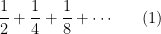
In this case, each term is one half the previous term, so that the ratio between successive terms is always 

This is the familiar math of the Dichotomy paradox from Zeno’s paradoxes.
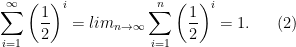
It is important to note that not every geometric series converges. If the number 

Let 

It is not hard to see why this is true:

Returning to the example of 


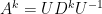
Matrices behave like numbers in some ways, for example they can be added and multiplied, yet quite differently in others. The generalization of geometric series as in Feizi et al. specifically deals with diagonalizable matrices, a class of matrices which has many convenient properties. Let 

Notice that what has changed is that the condition that 


In following Feizi et al., we call the number
In Feizi et al., the matrix A is called the “direct effect”, and the remainder of the sum the “indirect effect”. One should think of the indirect effect as consisting of echoes of the direct effect. Furthermore, following the language in Feizi et al., we call the rate at which the terms in the indirect effect decay the indirect flow. When it is strong, the terms decrease slowly. When it is weak, the terms decrease rapidly.
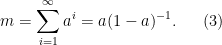
In number deconvolution the goal is to infer 


That is the formula for number deconvolution.
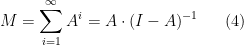
In network deconvolution the goal is to infer 


That is the formula for network deconvolution.
Everything looks great but there is a problem. Even though one can plug any number 


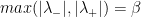
The restriction on 


But what if we wanted number deconvolution to work for all negative numbers? One idea is to follow Feizi et al.’s approach and introduce a scaling factor called 


When 


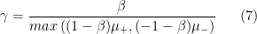
then the matrix 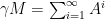

Matrices do behave differently than numbers, and so it is not true that network deconvolution can produce any matrix as an output. However, as with number deconvolution, it remains true that network deconvolution can produce an infinite number of possible matrices.
Not only do Feizi et al. not mention this anywhere in the main text, instead they create the impression that there is a single output from any input.
Feizi et al.’s response
We now turn to the response of Feizi et al. to our post. First, upon initial inspection of the “Try It Out” site, we were astounded to find that the code being distributed there is not the same as the code distributed with the paper (in particular, step 1 has been removed) and so it seems unlikely that it could be used to replicate the paper’s results. Unless, that is, the code originally distributed with the paper was not the code used to generate its results. Second, the “one click reproduction”s that the authors have now added do not actually start with the original data but instead merely produce plots from some results without showing how those results were generated. This is not what reproducibility means. Third, while the one matrix of results from a “one click reproduction” that we looked at (DI_ND_1bkr.mat) was very close to the matrix originally distributed with the paper, it was slightly different. It was close and hopefully it does generate basically the same figure, but as we explain below, we’ve spent a good bit of time on this and have no desire to spend any more. This is why we have tried to incentivize someone to simply reproduce the results.
In retrospect, we regret not explaining exactly how we came to be so skeptical about the reproducibility of the results in the Feizi et al. paper. While we very quickly (yet not instantly) recognized how misleading the paper is, our initial goal in looking at their results was not to verify reproducibility (which we assumed) but rather to explore how changing the parameters affected the results. Verifying that we could recover the results from the paper was only supposed to be the first step in this process. We downloaded the file of datasets and code provided by the authors and began examining the protein contact dataset.
After writing scripts that we verified exactly regenerated some figures from the paper from the output matrices distributed by the authors, we then checked whether we arrived at the same results when running the ND code on what we assumed was the input data (files with names like “MI_1bkr.txt” while the output was named “MI_ND_1bkr.txt”). We were surprised when the output did not match, however we were then informed by the authors that they had not distributed the input data but rather thresholded versions of the input. When we asked the authors to provide us with the actual data, we were told that it would violate scientific etiquette to send us another scientist’s dataset and that we would have to regenerate it ourselves. We had never heard this claimed point of etiquette before, but acquiesced and attempted to do so. However, the matrices produced from the original data were actually a different size than those used by the authors (suggesting that they had used a different alignment).
Stymied on that front, we turned to the DREAM5 dataset instead. While the actual scoring that goes into the DREAM analysis is fairly complicated, we decided that we would start by merely checking that we could regenerate the output provided by the authors. We eventually received step-by-step instructions for doing so and, because those steps did not produce the provided output, asked a simple question suggested by our experience with protein contact dataset: to generate the provided results, should we use as input the provided non-ND matrices? We asked this question four times in total without receiving a reply. We sent our script attempting to implement their steps and received no response.
At some point, we also discovered that the authors had been using different parameter values for different datasets without disclosing that to their readers. They could provide no coherent explanation for doing so. And sometime after this, we found that the authors had removed the data files from their website: readers were directed instead to acquire the datasets elsewhere and the results from the paper were no longer provided there.
At this point, we expect it is obvious why we were skeptical about the reproducibility of the results. Having said that, we never wanted to believe that the results of the paper were not reproducible. It was not our initial assumption and we still hope to be proven wrong. However, we continue to wait, and the fact that the code has been changed yet again, and that the authors’ explanation in regards to figure S4 does not appear to explain its changes (see below) do not fill us with confidence.
We repeat that while most of the discussion above has focused on replicability, we will quote again the definition of “fraud” used in the original post: “deception deliberately practiced in order to secure unfair or unlawful gain”. Our main point is this: would any honest reader of the main text of the original paper recognize the actual method implemented? We don’t think so, hence deception. And we believe the authors deliberately wrote the paper in this way to unfairly gain acceptance at Nature Biotechnology.
Now, in response to the authors rebuttal, we offer the following (Feizi et al. remarks in italics):
Point-by-point rebuttal
Appendix A
The pre-processing step that Bray and Pachter criticize (step 1 in their description of our work) has no effect on the performance of ND. Mathematically, because our matrices are non-negative with min zero, a linear scaling of the network results in a similar scaling of its eigenvalues, which are normalized during eigenvalue scaling, canceling out the linear scaling of step 1. Practically, removing step 1 from the code has little effect on the performance of ND on the DREAM5 regulatory networks, as we show in Figure 1 below.
We cannot imagine how the authors came to make the statement “our matrices are non-negative with min zero”. After all, one of the inputs they used in their paper was correlation matrices and they surely know that correlations can be negative. If the map in step 1 were linear rather than – as we correctly stated in the document they are responding to – affine (for those unfamiliar with the terms, “linear” here means only scaling values while “affine” means scaling and shifting as well), then this explanation would be correct and it would have no effect. This just makes it even stranger that immediately after giving this explanation, the authors produced a graph showing the (sometimes quite significant) effect of what we assume was the affine mapping.
Stranger still is that after this defense, Step 1 has now been removed from the code.
Appendix B
The eigenvalue scaling (step 5) is essential both theoretically, to guarantee the convergence of the Taylor series, and practically, as performance decreases without it in practice. This step is clearly stated in both the main text of our paper and in the supplement, despite the claims by Bray and Pachter that it somehow was maliciously concealed from our description of the method (just search the manuscript for the word ‘scaling’). Our empirical results confirm that this step is also necessary in practice, as ND without eigenvalue scaling is consistently performing worse, as we show in Figure 2 below:
We do not understand why the author’s felt the need to defend the use of eigenvalue scaling when we have never suggested it should be removed. Our objection was rather to how it was presented (or not) to the reader. Yes, there is a mention of the word “scaling”. But it is done so in a way that makes it sound as though it were some trivial issue: there’s an assumption, you scale, assumption satisfied, done. And this mention occurs in the context of the rest of the main text of the paper which presents a clear image of a simple, parameterless, 100% theoretically justified method: you have a matrix, you put it into the method, you get the output, done (and it is “globally optimal”). In other words, it is the math we discuss above prior to the arrival of the parameter 
Yes, scaling is dealt with at length in the supplement. Perhaps Feizi et al. think it is fine for the main text of a paper to convey such a different image from the truth contained in its supplement and in the code. We do not and we would hope the rest of the scientific community agrees with us.
Appendix C: Robustness to input parameters.
Bray and Pachter claim that “the reason for covering up the existence of parameters is that the parameters were tuned to obtain the results”. Once again the claims are incorrect and unfounded. (1) First, we did not cover up the existence of the parameters. (2) Second, we used exactly the exact same set of parameters for all 27 tested regulatory networks in the DREAM challenge. (3) Third, we show here that our results are robust to the parameter values, using β = 0.5 and β = 0.99 for the DREAM5 network.
(1) Again: in the main text of the paper, there is not even a hint that the method could have parameters. This is highly relevant information that a reader who is looking at its performance on datasets should have access to. That reader could then ask, e.g. what parameters were used and how they were selected. They would even have the ability to wonder if the parameters were tuned to improve apparent performance. It is worth noting that when the paper was peer reviewed, the reviewers did not have access to the actual values of the parameters used.
(2) It is, of course, perfectly possible to tune parameters while using those same parameters on multiple datasets.
(3) The authors seem to have forgotten that there are two parameters to the method and that they gave the other parameter (alpha) different values on different datasets as well. They also have omitted their performance on the “Community” dataset for some reason.
Appendix D: Network Deconvolution vs. Partial Correlation.
Bray and Pachter compare network deconvolution to partial correlation using a test dataset built using a partial correlation model. In this very artificial setting, it is thus not surprising that partial correlation performs better, as it exactly matches the process that generated the data in the first place. To demonstrate the superiority of partial correlation, Bray and Pachter should test it on real datasets, such as the ones provided as part of the DREAM5 benchmarks . In our experience, partial correlation performed very poorly in practice, but we encourage Bray and Pachter to try it for themselves.
We looked at partial correlations here for a very simple reason: the authors originally claimed that their method reduced to it in the context we considered here. Thus, comparing them seemed a natural thing to do.
The idea that we should look at the performance of partial correlations in other contexts makes no sense: we have never claimed that it is the right tool to solve every problem. Indeed, it was the authors who claimed that their tool was “widely applicable”. By arguing for domain specific tools, they seem to be making our point for us.
Claim 1: “the method used to obtain the results in the paper is completely different than the idealized version sold in the main text of the paper”.
The paper clearly describes both the key matrix operation (“step 6” in Lior Pachter’s blog post) which is shown in figure 1, and all the pre- and post-processing steps, which are all part of our method. There is nothing mischievous about including these pre- and post-processing steps that were clearly defined, well described, and implemented in the provided code.
The statement that the paper describes all steps is simply false. For example, the affine mapping appears nowhere.
Claim 2: “the method actually used has parameters that need to be set, yet no approach to setting them is provided”.
It is unfortunate that so many methods in our field have parameters associated with them, but we are not the first method to have them. However, we do provide guidelines for setting these in the supplement.
It is strange to suggest that it is unfortunate that methods have parameters. It is also strange to describe their guidelines as such when they did not even follow them. Also, there is no guideline for setting alpha in the supplement. In their FAQ, they say “we used beta=0.5 as we expected indirect flows to be propagating more slowly”. We wonder where one derives these expectations from.
Dr. Pachter also points out that a correction to Supplement Figure S4 on August 26th 2013 was not fully documented. We apologize for the omission and provide additional details in an updated correction notice dated February 12, 2014.
The correction notice states that the original Figure S4 was plotted with the incorrect x-axis. In particular it states that the maximum eigenvalue of the observed network was used, instead of the maximum eigenvalue of the direct network. We checked this correction, and have produced below the old curve and the new curve plotted on the same x-axis:

The new and old Figure S4. The old curve, remapped into the correct x-axis coordinates is shown in red. The new curve is shown in blue. Raw data was extracted from the supplement PDFs using WebPlotDigitizer.
As can be seen, the two curves are not the same. While it is expected that due to the transformation the red curve should not cover the whole x-axis, if the only difference was the choice of coordinates, the curves should overlap exactly. We cannot explain the discrepancy.

32 comments
Comments feed for this article
February 18, 2014 at 5:16 am
Paul
Your result for the application of eq. (3) to 1/2 has a typo. And some latex formulas don’t parse yet but presumably you know that already.
I was pointed to your blog an hour ago and became a fan almost instantly.
February 18, 2014 at 5:23 am
Lior Pachter
Thanks- I think the issues should be fixed now.
February 18, 2014 at 6:36 am
Florian
Your result from application of eq (5) to m=-2 seems wrong as well: one gets a=2 and not a=1.
Very nice article.
February 18, 2014 at 9:08 am
Lior Pachter
Thanks! At the end I re-indexed all the geometric sums from 1 instead of 0 to be consistent with Feizi et al. and introduced some typos. Thanks for reading carefully.
February 19, 2014 at 9:28 pm
village-idiot
aren’t you glad that these people are politely pointing out errors as typos, and not accusing you of fraud, as you might have done?
February 19, 2014 at 9:33 pm
Lior Pachter
Actually, all the errors fixed in the August 26th supplement of Feizi et al. were fixed thanks to us (for example equation 12 in their supplement, in which they originally had an error that we pointed out). I think its clear in our posts that our accusation of fraud is not about error, but about them deliberately misleading their readers and the journal for unfair gain.
February 18, 2014 at 7:40 am
Manolis Kellis
We are disappointed that Pachter will not retract his allegations. He now claims that “The distance between the main text and the method is simply too great”. We continue to disagree, and we stand firmly by the specific presentation of our work, with a broadly accessible main text that consistently refers to a much more formal and detailed supplement. We will not continue responding to his inaccurate descriptions and deceiving allegations, and instead let our work speak for itself. We are proud of our paper and method, and we encourage you to read it and apply it broadly.
February 18, 2014 at 7:50 am
AnonOpt
Regarding the discrepancy between the old and new S4 figure, I want to note that the performance according to their new figure is worse than that according to their old figure.
While I agree that results (especially in a computational context) should ideally be completely reproducible from the available code and data, the above (along with many other things like their willingness especially compared to many other authors to provide their code, etc.) indicates more that they are at worst guilty of overhyping their results rather than anything close to fraud.
I also agree that ideally, scientists would not overhype results and present all caveats to their method in the main text, but the current incentives do not always support that.
A large number of scientists (and not just in compbio) hype up their results and I feel it’s unfair to pick on a single person for that.
February 18, 2014 at 10:23 am
RobertA
I disagree with the above comment. Having dipped my toes with a similar field before retreating to a more technical field quickly, I can assert that such behavior (overhyping as you call it, fraud as Lior calls it) does cause damage. Its repeated use leads to a field where you end up not judging the work, but judging the name of the institution, the tone of the paper (assertive and grandiose is better), the prettiness of the package etc. Consequently, you can game the system and focus the attention of the research community on worthless subjects to satisfy your vanity.
Now while I think that Lior’s making a good point, I am also sure that many many people, the authors of the paper included, _genuinely_ feel it is not fraud. To wit, their proud revelation that Lior did not teach them anything in his review of the paper. The authors knew about the combinatorial artifacts, had written about it, but did not put it in the published paper because … ? What was used as a rebuttal point by them is in fact the most damning evidence of fraud to date, at least in my book.
February 18, 2014 at 12:51 pm
AnonOpt
I completely agree with you that overhyping needs to be corrected. I think much better reviewing is one of the ways that can be accomplished. But I feel that a lot of other scientists are guilty of similar behavior as Manolis in that regard and thus I’m uncomfortable singling out one person.
I agree the combinatorial artifact part is troubling. Once they learned of the issue, they should have atleast had a table demonstrating how clustered the solutions found by their algorithm usually were compared to a clique-finder, etc.
Here I’d like to note a very well known paper (Clustering of Time Series Subsequences is Meaningless: Implications for Previous and Future Research) where a somewhat similar issue is discussed in the context of time series. The authors go on to present algorithms that avoid the issues discussed. The paper has had a very lasting impact on the field and if Grochow & Kellis had decided to go in that direction, that may have worked out better for them and definitely for the scientific community.
February 18, 2014 at 2:07 pm
A N
Overhyping the results is wrong. Bash M. Kellis.
Overhyping the errors is Ok. Praise L. Pachter.
February 18, 2014 at 10:53 pm
Norman Yarvin
Fraud is a legal term. It carries an implication that someone should go to prison, rather than, say, just being defunded and banished from the scientific community.
February 18, 2014 at 11:58 pm
homolog.us
“It carries an implication that someone should go to prison”
Or gets promoted, if he works for a TBTF bank 🙂
Context matters.
February 19, 2014 at 2:07 am
Saheli
Fraud *can* be a legal term, but that doesn’t mean it always is. Lior was pretty clear about the definition he was using, which came from freedictionary.com: unlawful OR unfair. An act may be considered ethically fraudulent (i.e. unfair) even if it’s not *legally* fraudulent, and scientific fraud would describe a subset of such acts.
February 19, 2014 at 12:15 pm
Norman Yarvin
Still, if he had said “unmitigated sleaze”, he wouldn’t have had to explain himself.
February 18, 2014 at 11:01 pm
Rob
Which errors? Errors are fine [well, not really, but not morally objectionable], willful hiding of _very_ relevant facts about your methods is not fine. [And, pardon me if I reiterate, but the admission that they knew about the combinatorial artifacts was really a low point here]. I think that this is what it is all about. If you want to understand it as overhyping errors, then you are deluding yourself. If you meant to say: it is unfair to pick on Kellis, since by opening any issue of Nature Bio tech or other ‘leading’ journal, you would observe similarly compromised papers, then I might agree.
February 23, 2014 at 12:05 pm
Marnie Dunsmore
Lior,
I would like to make an appointment to come to talk to you. Do you have an email address? I haven’t been able to find it. Alternatively, when are your office hours?
February 23, 2014 at 12:55 pm
Lior Pachter
My contact info is here:
http://math.berkeley.edu/~lpachter/contact.html
I’ll be happy to meet with you- just send me an email.
February 23, 2014 at 1:35 pm
Marnie Dunsmore
Got it. Sending email now.
February 25, 2014 at 10:10 am
PaulR
I feel very skeptical of the idea that it is possible to write the observed interactions as the sum of powers of the real interaction matrix. In the supplementary information the authors write:
“Network deconvolution assumes that networks are linear time-invariant flow-preserving operators which excludes nonlinear dynamic networks as well as hidden sinks or sources. Under this condition, indirect flows over different paths are modeled by using power series of the direct matrix, while observed dependencies are modeled as the sum of direct and indirect effects.”
Ie: it makes sense to add and multiply the measures of interaction.
I’m happy that if a measure of interaction satisfies the above then (ignoring lack of convergence[!!] of the geometric series) the proposed idea sounds plausible.
However, the authors appear not to have proven that the above assumptions hold with correlation coefficients or mutual information. If that assumption does not hold with the measures of interaction used to construct the networks then the idea of “adding” or “multiplying” edge weights is nonsense (for example, it does not make sense to multiply mutual information together to get mutual information, or add correlation coefficients together to get correlation coefficients).
Before instructing the community to use the method “broadly” I believe that the authors should first prove that the assumptions are met by the plethora of methods used to construct networks and the quantities represented by the edge-weights.
February 27, 2014 at 2:29 pm
garance
I am a neutral observer. I think Manolis should clarify the situation by telling Lior exactly how to reproduce the results in his paper. Such transparency seems like an obvious solution. All published scientific work should be reproducible and if Manolis is worried about releasing his collaborators’ data, surely he can send it to Lior alone. I have great respect for both the Kellis and Pachter labs, but without the full story, it’s very difficult to arrive at any conclusion and the Kellis lab will have to live under a shadow of scrutiny.
March 1, 2014 at 12:02 pm
anon
The right hand side of equation 2 should start from i equal to 1.
March 3, 2014 at 8:52 pm
LJO
Pachter’s blog posts are very damning on first read. But after reading the paper, the charge of “fraud” seems gratuitous. While the lack of transparency raises questions, and of course the omission in the revision note is embarassing, Pachter’s allegation is not of mere sloppiness and opaqueness.
First, it does not appear that the authors have attempted to cover up the importance of the scaling. The fifth sentence of the Methods section is “Note that, the observed dependency matrix is linearly scaled so that the largest absolute eigenvalue of G_dir < 1," and most of the second paragraph deals with this scaling. Though the parameter beta is not mentioned directly, it is totally clear that preprocessing is required: "G_obs can be derived…" clearly implies that the input matrix is not just the original adjacency matrix. There is no deception here.
Second, whereas the "number deconvolution" analogy makes the scaling appear very illegitimate, it seems natural that such a step would be necessary for an adjacency matrix whose scale may be arbitrary in the first place. No sophisticated data analysis tool is a black box, and nothing in the paper suggests that ND should be used as such. Rescaling is the natural way to address the fact that the magnitude of a second-order effect as defined by transitive closure, compared with the magnitude of the first order effects, is scale dependent. This is most obvious going in the reverse direction: Given a binary matrix of direct interactions H_dir, if we wish to perform transitive closure, H_dir must be scaled down so that second order effects have smaller size than first order effects (and even if H+H^2+… already converges the scale may be wrong). The natural way is to take G_dir=const*H_dir. Given H_obs on the scale of H_dir, it is appropriate to take G_obs=const*H_obs, and G_dir=G_obs(1+G_obs)^-1. The scaling parameter is intuitively necessary, and its presence does not diminish the justifiability of the method.
Grasping the necessity of scaling and closely reading paragraphs 1-2 of Methods, there is no evidence of fraud. ND might be slightly more ad hoc than Fig. 1 makes it seem, but it is based on a theoretically sound idea and Fig. S4 shows that it is fairly robust in practice. The "gap between the main text and the method" is not "too great" but rather, much too small to support the heavy allegation of fraud.
March 3, 2014 at 9:06 pm
Lior Pachter
Thanks for your comment, and for taking the time to write a thoughtful response to our allegations.
Unfortunately I don’t understand your claim that “the scaling parameter is intuitively necessary, and its presence does not diminish the justifiability of the method.” The point of the “number deconvolution” post was to make it clear, that once scaling is introduced into the model, there are an infinite number of possible solutions to the inverse problem. Without knowledge of how the observed matrices were scaled, how is one supposed to figure out how to scale? The authors themselves provide no theoretical or practical approach to scaling, other than to offer, on their FAQ: ” For the regulatory network, we used beta=0.5 as we expected indirect flows to be propagating more slowly” (it should be noted that even that was posted only recently as a response to our blog post). In the original paper seen by the reviewers and published on July 16th, aside from a single sentence in the main paper, there was only an explanation and demonstration in the supplement suggesting it should always be set (close) to 1, thereby implying it wasn’t really a parameter at all. This was a lie. Its really not accurate to say its “slightly more ad hoc than Fig. 1 makes it seem”. Figure 1 is not ad hoc at all, whereas the method is not ad hoc, but incoherent.
As you say yourself, I think there is a very big difference between publishing a paper with errors or oversights, as opposed to deliberately brushing a significant and problematic issue under the rug so that reviewers and readers don’t catch on to it. To make the point concrete, of how serious of a problem the scaling factor is, suppose you actually wanted to use ND tomorrow on a problem where you did not already know what the answer should be. How would you choose your scaling factor to improve your network? How would you know the choice you did pick improved it at all as opposed to degrading its quality. Would you really use ND having understood what I explain in my post?
March 4, 2014 at 1:23 am
Nicolas Bray
First, it does not appear that the authors have attempted to cover up the importance of the scaling. The fifth sentence of the Methods section is “Note that, the observed dependency matrix is linearly scaled so that the largest absolute eigenvalue of G_dir < 1,"
It’s not the importance of scaling (or rather its existence) that we suggested was covered up but rather its implications. Really, is this not a truly bizarre way to, effectively, introduce a parameter? It’s phrased as though this were some minor technical detail rather than something which seriously problematizes the nice clean picture they portray in their main figure on the method. When I first read that sentence, it took me a minute to realize that different scalings will give different results and I’m apparently considerably more familiar with this type of material than most readers.
A normal way to write that would have been “The observed dependency matrix is linearly scaled so that the largest absolute eigenvalue of G_dir is equal to β, a parameter of the method.” But at that point, the reader would probably like to know how this parameter is set, how it affects the results, and all that other murky stuff.
No, better not to mention it.
Though the parameter beta is not mentioned directly, it is totally clear that preprocessing is required: “G_obs can be derived…” clearly implies that the input matrix is not just the original adjacency matrix.
That sentence is referring to the original calculation of G_obs from data, e.g. by taking correlations between gene expression measurements. I’m not sure what you’re referring to by “the original adjacency matrix” but that’s as original as it gets here.
Regarding your “Second,”, I see you’ve phrased everything in terms of adjacency matrices and transitive closures. While the authors did say things like, “transitive closure of a weighted adjacency matrix”, as far as I can tell, there is no commonly accepted notion of such a thing. And, yes, it’s for the same reasons we’ve been discussing here: under the two definitions that Feizi et al. could be using here, either there are either some matrices which don’t have a transitive closure or every matrix has infinitely many. But the fact that their notion of “transitive closure” has exactly the same problems is another fault of the paper, not a defense. (We possibly should have brought this up in the original post but there were so much strange things going on, we couldn’t address it all.)
Given a binary matrix of direct interactions H_dir, if we wish to perform transitive closure, H_dir must be scaled down so that second order effects have smaller size than first order effects (and even if H+H^2+… already converges the scale may be wrong). The natural way is to take G_dir=const*H_dir. Given H_obs on the scale of H_dir, it is appropriate to take G_obs=const*H_obs, and G_dir=G_obs(1+G_obs)^-1.
While I’m not sure what you might mean by “(and even if H+H^2+… already converges the scale may be wrong)” or “Given H_obs on the scale of H_dir”, you’ve written both G_dir=const*H_dir and G_dir = G_obs(1+G_obs)^-1, which might lead someone to conclude that const*H_dir = G_obs(1+G_obs)^-1. So I’d just like to note that that is not correct.
You appear to have some notion of “transitive closure” which is even more particular than anything hinted at in Feizi et al. But whatever your notion is, surely you’ll agree that what you’re doing there is not, in fact, inverting it: you began with H_dir and your end result is not H_dir. This would be in contrast to Feizi et al. where we find statements such as “network deconvolution takes a global approach by directly inverting the transitive closure of the true network.”
That statement is absolutely false. And the authors must have known it was false.
Do you really consider this to be acceptable behaviour?
March 4, 2014 at 9:17 am
LJO
What I mean by “H_obs on the scale of H_dir” is precisely that H_obs=1/const*G_obs, and yes, trivially, then const*H_dir=G_obs(1+G_obs)^-1. I should clarify scale to mean units: the linear flow assumption implies that there is a relation on the units, u^2=u. That way, matrix multiplication makes sense when you do TC. But if your scale is wrong, it is false that (u/const)^2=u/const. This is what I mean that the rescaling is natural, and why I disagree that it “seriously problematizes” anything beyond the original flow assumption. The paper is somewhat opaque, sure, but fraudulent? I do not buy that clarifying this issue would have led to the paper’s rejection by Nature Biotech.
March 4, 2014 at 10:23 am
Nicolas Bray
Actually, your example is even more confusing than I originally noticed, e.g. you have H_obs and G_obs but only one matrix is being observed in this context so I’m not sure what exactly you’re doing here. If you’d like to write it out in more detail, then we could actually go over the math but one thing I can guarantee you is that if the matrix is scaled after performing the geometric sum* then you will not recover the original matrix up to a constant factor by the operation A(I + A)^-1. That operation is non-linear and so a linear scaling of A has a non-linear effect on the output.
About the discussion of units, I’m again somewhat confused. Of course there is no unit u for which u^2 = u. If there were, dimensional analysis would have some serious problems.
The introduction of scaling takes you from a scenario where every possible input matrix to the method has a unique output to one where every input matrix has an infinite number of possible outputs, depending on the value of a parameter. If you don’t think that’s the kind of thing that a reader might like to know about, I really don’t know what to tell you.
And while I let this slide before because your comment was mostly actual content rather than opinion, if you are going to be offering your personal opinions about the paper, you really really ought to disclose the fact that you have a direct relationship with one of the authors of the paper. To fail to do so would be…”somewhat opaque”, at best.
(* Please, let’s not use the term “transitive closure” since that term actually has an accepted meaning in other contexts.)
March 4, 2014 at 10:31 am
Nicolas Bray
PS. I forgot to respond previously to your statement that “[ND] is based on a theoretically sound idea”. You need to keep in mind that what Feizi et al. did here is propose a model for indirect effects and then give a method which kind of does something like recovering direct effects within that model (it doesn’t even really do that, of course).
So ND is only even plausibly “theoretically sound” when applied to data that actually arises from their model and yet the authors have not given even a single example where their model actually applies. As another commenter pointed out, it’s fairly obvious that, e.g., mutual information will not behave in the way described by this model.
A more accurate statement would be that ND is a heuristic method based on an intuitive, but theoretically unjustified, idea.
March 4, 2014 at 4:02 pm
LJO
Thank you– I should say that I am an undergraduate working with Soheil and indirectly with Manolis (however, I have not spoken with them about this issue, and do not speak for them at all).
Okay, now let’s try this again. From the main text (and the Fig. 1 caption) of Feizi et al:
“Our formulation of network deconvolution has two underlying modeling assumptions: first that indirect flow weights can be approximated as the product of direct edge weights, and second, that observed edge weights are the sum of direct and indirect flows. When these assumptions hold, network deconvolution provides an exact closed-form solution for completely removing all indirect flow effects and inferring all direct interactions and weights exactly (Fig. 1d). We show that network deconvolution performs well even when these assumptions do not hold…”
My point was precisely that this this assumption is dependent on scale, as you understand: if H_dir=1/const*G_dir, then it is false that const*H_dir(1-H_dir)^-1=G_dir(1-G_dir)^-1. Conversely, if H_obs=1/const*G_dir(1-G_dir)^-1 , then it is false that H_dir=H_obs(1+H_obs)^-1.
Thus, the criticism that the choice of beta is arbitrary is a subset of the criticism that there is no unique, optimal transformation that will as nearly as possible satisfy the model assumptions. But the authors do not claim that there is such. They only claim that their method is exact when the assumptions hold (true, though the hypothetical is unlikely) and that it still works well when the assumptions do not hold (also true).
Now if ND were not robust to the choice of beta, and there were no good heuristic to choose it, then it might not be true that ND works well in practice when the flow assumptions fail (without being able to overfit the parameter, that is). But in fact ND turns out to be robust to the choice of beta (http://compbio.mit.edu/nd/ND_beta_effect.pdf). Unlike “number deconvolution,” in which different choices of the scaling parameter lead to totally different results, in ND, choices as disparate as .5 and .99 produce similarly good results. Basically, it appears that as long as the much weaker eigenvalue/convergence assumption is satisfied, the method performs well.
Is the parameter beta a deep dark secret that discredits the whole method, or a preprocessing detail used to help satisfy the well-documented model assumptions?
March 4, 2014 at 9:39 am
LJO
In addition, it turns out that the algorithm is in fact robust to the choice of beta, and Pachter’s accusation that beta was fine-tuned to produce the results for the DREAM5 networks is not substantiated. http://compbio.mit.edu/nd/ND_beta_effect.pdf
March 5, 2014 at 7:42 am
Lior Pachter
Dear LJO,
It is impossible to have a meaningful discussion about mathematics, when sentences are used that don’t mean anything. For example, you write that
“Thus, the criticism that the choice of beta is arbitrary is a subset of the criticism that there is no unique, optimal transformation that will as nearly as possible satisfy the model assumptions.”
What are you talking about? What “optimality” are you referring to here? what does “nearly as possible” mean? What model are you talking about? The model that includes scaling as a parameter, or the one that doesn’t?
The math in the Feizi et al. is not complicated. But the paper itself describes methods exactly as you have above, which is precisely part of the fraud, because it leads people to be confused about a very simple fact: the actual model of Feizi et al. has a parameter, beta, and there is no way to know how to set it. Yes, that is is a dark secret of the paper (by the way alpha is another).
I am not willing to give Feizi et al. the benefit of the doubt that they disclosed beta because the main text of the paper was deliberately written to mask it. Even the supplement section 1.3 now presents it in an oblique way, where they write “This assumption can be satisfied by lin- early scaling the observed dependency matrix. “Its not an assumption (!!) Its a parameter (!!) Second, the idea that the method is “robust to beta” is ludicrous. There are an infinite number of possible matrices that can come out of the method depending on beta, including the original input(!) Third, the results are not reproducible- not even the authors have claimed the $100 I’m offering. And, why haven’t they offered an explanation for why Figure S4 does not actually match the original one (even after transforming the x-axis which they claim was the issue).
I have one final thought (experiment) to leave you with. Suppose network deconvolution (whatever it actually is) works as you think it might. Its robust to some minor pre-processing (beta), and alpha also just doesn’t matter. Nothing matters. Whatever… network deconvolution is just a good thing to plug a matrix into it- you always get out a better one and biologists should start using it. Lets go with that story for a second. So I come with my matrix and I run the ND.m code and I got a better one. Now, I have a new matrix, and I’m thinking running it through ND.m again will make it even better right? I mean network deconvolution, in your belief system, doesn’t make things worse, and it doesn’t really matter where the matrix that is being inputted came from in the first place. Mutual information, correlation matrices, coauthorship networks, or the adjacency matrix of a graph. Its all just good stuff to plug into he thing. Great. Lets do it a third time to clean up even more. And a fourth time. Lets run network deconvolution over and over to clean the original matrix spick and span… not just a superficial dusting by running it once. After all, it may take more than one round to truly get rid of the pesky indirect effect. The authors themselves admit straight out that a single run of ND.m doesn’t clean out all the indirect effect. In our Gaussian graphical model example they admit openly that there are better optimal methods for specific domains and settings (e.g. partial correlation). But their argument is that deconvolution is just a good thing to do and doesn’t hurt.
Please don’t just think about my experiment, try it…
P.S. I truly appreciate both your effort to work through figuring out the paper, and also your public disclosure of who you are. When you apply to graduate school (if you are not completely jaded after being exposed to the people involved in this horrible affair), please do consider Berkeley. I’m serious.
September 20, 2014 at 6:47 pm
台灣大樂透
Amazing article, thank You !!